Filtering | Academy of EMC

13 Filtering

Filter Fundamenals

Low-Pass Filters

Low-Pass Filters.

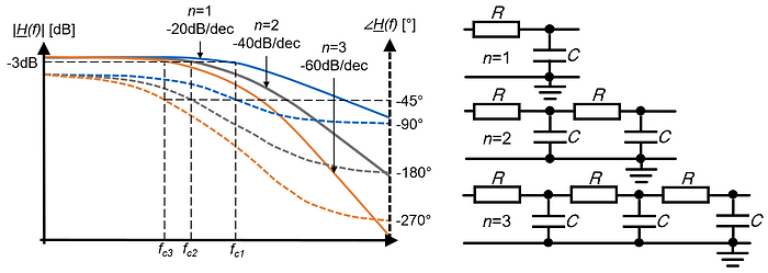
Low-pass filters are the most common filters in the world of EMI and EMC. They reject undesired HF energy above a desired cut-off frequency fc [Hz]. The figure below shows the frequency response of ideal low-pass filters (skin effect, stray capacitance, and other nonlinearities are neglected). At the cut-off frequency fc [Hz], the insertion loss is 3dB and the phase shift is -􀀀45°. The attenuation for frequencies f>fc is n⋅20dB and the maximum phase shift of a low-pass filter is n⋅90deg, where n is the filter order.

The filter performance (e.g., cut-off frequency fc [Hz]) depends not only on the filter components themselves but also on the source impedance Zsource [Ω] and the load impedance Zload [Ω]. Therefore, the input and output impedances of the filter should be matched in the useful frequency range and mismatched in the EMI noise frequency range.

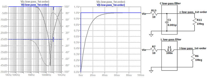
It is highly recommended to simulate EMI analog circuit board filters with the real-world source and load impedances and the non-ideal SPICE models of the filter elements. The LTSpice simulations of the low-pass filters below show that it is important to consider the non-ideal filter components (not the ideal components) because the non-ideal behavior of capacitors, inductors, and ferrite beads influence the filter performance significantly at high frequencies.

SPICE simulation 1st order low-pass filter

In EMC, filtering helps to minimize emissions of a product and increase the product’s immunity against electromagnetic interference. The topics are important to understand for a good EMC design.

Filter Fundamentals.

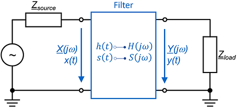
A linear and time-invariant (LTI) filter can be characterized in the time- and the frequency-domain:

Time-domain. In the time domain, a filter can be characterized by its impulse response h(t) or its step response s(t).
Frequency-domain. In the frequency domain, a filter can be characterized by its frequency response H(jω) (Fourier transform, bode plot).

On this website, we focus on filters that are causal LTI-systems (except for the non-linear transient filters for ESD/burst/surge and some non-linear digital algorithms). LTI-systems can be completely characterized by one of these functions [13.1]:

Impulse response h(t)
Step response s(t)
Transfer function H(s)

Causal, linear, and time-invariant (LTI) means:

Causal. A system is causal if the output depends only on present and past but not on future input values.
Linear. A system is linear if the output y(t) is a linear mapping of the input x(t). If a and b are constants, the output for a⋅x(t) is a⋅y(t) and b⋅y(t) for b⋅x(t). In addition, for linear systems, you can apply the principle of superposition (the output y for the input x=a⋅x1+b⋅x2 is y=a⋅y1+b⋅y2).
Time-invariant. A system is time-invariant when the output y(t) for a given input x(t) does not depend on whether x(t) is applied now or after a time T [sec]. If the output for x(t) is y(t), then the output for x(t-􀀀T) is y(t-􀀀T).

Note: Real-world components show non-linear effects, e.g., due to current saturation I [A] (inductors, ferrites) or non-ideal high-frequency behavior (inductors, capacitors). Therefore, real-world filters are only linear for certain operating conditions. The non-linearities and other undesired effects of filter components are described on our website about components. On this webpage, we assume that the filter components are used in their linear operating region.

Time-Domain: Step Response.

The goal of a filter characterization in the time-domain is to determine signal distortions and the time delay caused by the filter. Typical dime-domain input signals for characterizing a filter are:

Impulse Dirac delta function δ(t).
Unit step function u(t).

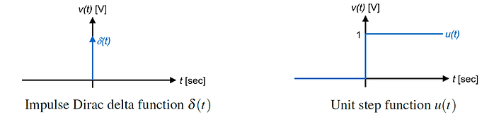
Impulse Dirac delta function vs. Unit step function.

If the input signal x(t) of an LTI-system is the Dirac delta δ(t) function:

then the output is defined as the impulse response h(t). The impulse response characterizes an LTI-system entirely and for any given input signal x(t) the output y(t) can be calculated as [13.1]:

Inpulse response time domain equation (convolution)

where, y(t) is the output signal from an LTI-system, h(t) is the impulse response of the LTI-system, x(t) is the input signal to an LTI-system and * is the convolution operator (a mathematical operation of two functions).

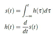
In practice, the step response s(t) (and not the impulse response h(t)) is usually used to characterize a filter [13.1]:

If the input is the unit step: x(t)=u(t), the output y(t) is called step response s(t). The step response s(t) can be calculated by integrating the impulse response h(t) and the impulse response h(t) by taking the derivative of the step response s(t) [13.1]:

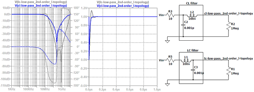
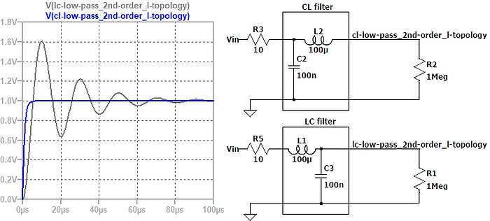
Calculate step response based on impulse response and vice versa

The figure below shows the step responses of two different low-pass filters, where:

Step signal amplitude u(t)=1V for t>0sec
Low source impedance Zsource=RS1=RS2=10Ω
High load impedance Zload=RL1=RL2=1MΩ
Filter type = 2nd order passive low-pass filter
Filter topology = L-topology

The simulated step responses (with LTSpice) below show that even passive low-pass filters can cause a significant amount of ringing and time delay. Therefore, it is always necessary to also check the time-domain behavior of an EMI-filter, not just in the frequency-domain behavior.

Step response simulation of two 2nd-order low-pass filters

Frequency-Domain: Frequency Response.

The frequency response H(jω) (Fourier transform) is the transfer function H(s) (Laplace transform, s=σ+jω) of a filter for a sinusoidal input signal, meaning s=jω. The frequency response H(jω) describes the attenuation in [dB] and the phase shift in [rad] or [°] as a function of frequency ω=2πf.

The Fourier transform of the filter’s impulse response h(t) is the frequency response H(jω) of the filter [13.1]:

The frequency response characterizes a filter in the frequency-domain. For any given
input signal X(jω), the output signal Y(jω) can be calculated as [13.1]:

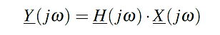
where, Y(jω) is the output signal of the filter, H(jω) is the frequency response of the filter, X(jω) is the input signal of the filter and ω [rad/sec] is the angular frequency of the sinusoidal input signal.

The frequency response H(jω) can also be calculated by using the Fourier transform of the step response S(jω):

Fourier transform of the step response and impulse response

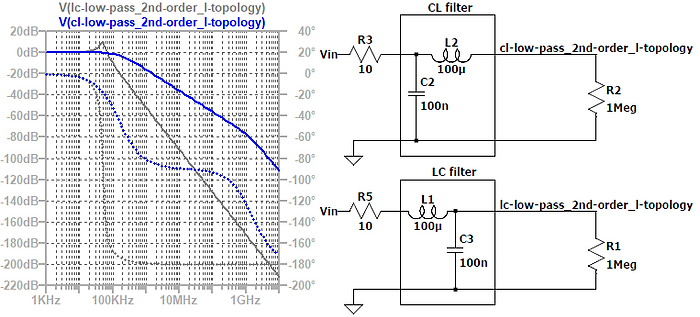
In practice, the frequency response H(jω) is shown in the form of a Bode plot. The figure below presents the Bode plot of the identical LC-lowpass-filters from above. The Bode plot shows us the following:

Ringing and resonance. It can be seen that the ringing in the time-domain matches the resonance in the frequency-domain at roughly fr=50kHz.
Order vs. attenuation and phase shift. The number of reactive components gives the order n of an analog filter; in other words: the sum of inductors L [H] and capacitors C [F] of the filter is equal to the filter order n. Because the filers are of second-order (n=2), the attenuation after the cut-off frequency is n⋅20dB=40dB and the maximum phase shift is n⋅􀀀90deg=􀀀180deg.
Source and load impedance vs. filter performance. The filter performance (attenuation, phase shift) depends on the filter components themselves and the source and load impedances.

Filtering_LCLowPass2ndOrderLTopology_FrequencyResponse.png

EMI filters should always be characterized by their step response (time-domain) and their frequency response (frequency-domain).

Time-domain. Determine distortion and time delay caused by the EMI filter.
Frequency-domain. Determine attenuate [dB] and phase shift of the EMI filter.

Analog filters: Time-domain vs. frequency-domain.

Active vs. Passive Filters

Active vs Passive Filters.

The low-pass filters in the previous section were all passive filters. If operational amplifiers or transistors are part of a filter, it is called an active filter. In most cases, EMI-filters are passive filters because the advantages of active filters mentioned in the table below are often not needed for EMI-filter applications.

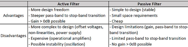
The figure below compares two second-order passive and active low-pass filters. Although, the active filter shows a narrower transition between the pass-band to the stop-band, the attenuation of the active filter at frequencies of f>100MHz is not as large as in the case of the passive filter and the active filter shows significant ringing in the time-domain. This example should just illustrate that an active filter is not always better than a passive filter; it all depends on the application’s requirements.

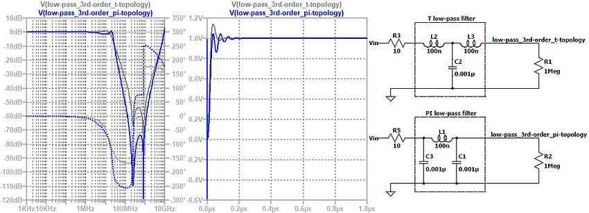
EMI RF filters are in most cases passive low-pass filters as shown in the figure below. In addition, the figure below helps you to choose the right filter topology (T-topology, L-topology, or PI-topology) depending on the source and load impedance.

Differential-Mode Filters

Differential-Mode Filters.

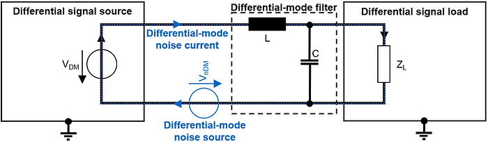
The filter components and topology for differential- and common-mode filters are not identical. Therefore, it is necessary to know if you deal with differential-mode or common-mode noise or both. Differential-mode noise filters are filters between a power or signal line and its return current line (see figure below). Typical differential-mode noise filter components are:

X-Capacitors.
Inductors.
PCB mount ferrite beads.

Common-Mode Filters

Common-Mode Filters.

Common-mode noise filters have the purpose to attenuate common-mode noise. An example of a common-mode filter is given in the figure below. Typical common-mode noise filter components are:

Y-capacitors.
Common-mode chokes.
Cable mount ferrite beads.

Mans Supply Filters

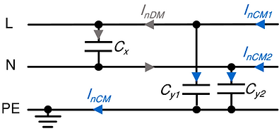
Mains Supply Filters.

Special care must be taken regarding the safety requirements of filter components of (public) mains supply filters. This is especially true for the X- and Y-capacitors (see figure below):

X-capacitors. X-capacitors are capacitors between line (L) and neutral (N) of the AC mains. A failure (short circuit of the X-capacitor) could result in fire.
Y-capacitors. Y-capacitors are capacitors between line (L) to ground and between neutral (N) to ground of the AC mains. The capacitance of a Y-capacitor must be low enough so that the maximum allowed leakage current through the Y-capacitor is below the required limit!

The classification of X- and Y-capacitors according to IEC 60384-14 is shown in the tables below.

In addition, the applicable safety standards of specific products must be considered. Examples are:

IEC 61010-1. Safety requirements for electrical equipment for measurement, control, and laboratory use - Part 1: General requirements.
IEC 62368-1. Audio/video, information and communication technology equipment - Part 1: Safety requirements.
IEC 62477-1. Safety requirements for power electronic converter systems and equipment - Part 1: General.

Transient Suppression Filters

Transient Suppression Filters.

A distinction is made between these three types of high-voltage transients:

Electrostatic discharge (ESD). Low energy pulses, very short rise-time.
Electrical fast transients (EFT). Bursts of low energy pulses, short rise-time.
Lightning surge pulses (surge). High energy pulses, medium rise-time.

The table below gives an overview of the three types of high-voltage transients.

ESD, burst, surge. Overview. Comparison.

The rise-time and the pulse energy are the most important parameters of voltage transients. The rise-times and the approximate(!) maximum pulse energy for ESD, EFT and surge are presented below [13.2].

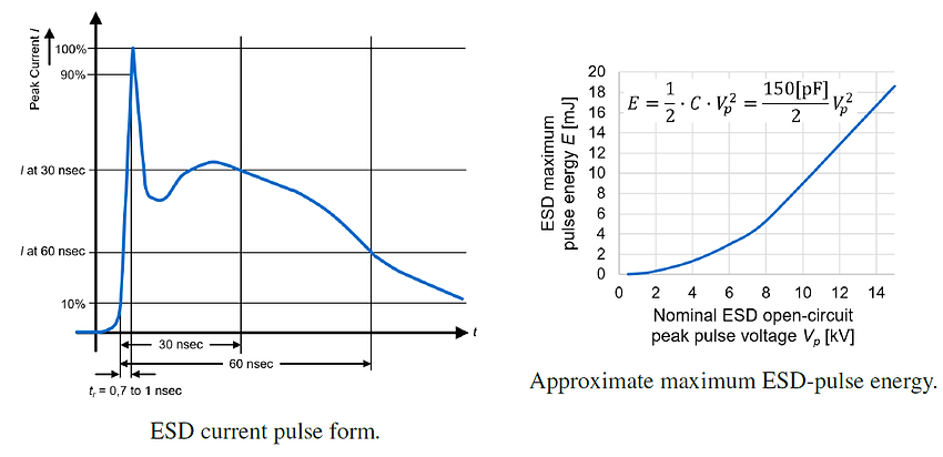
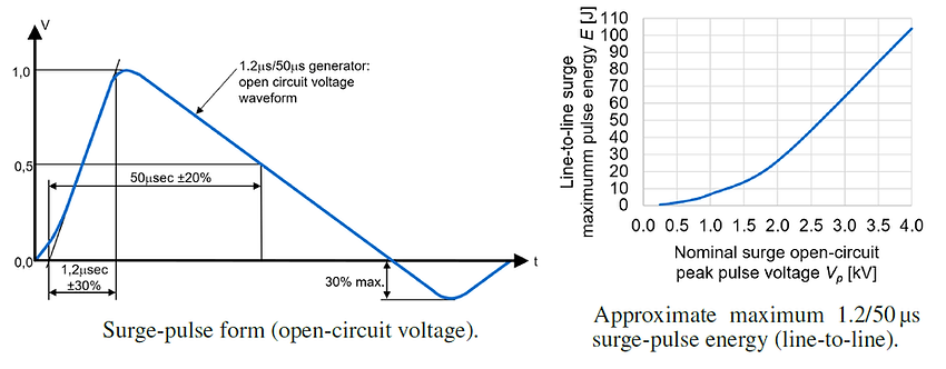
Surge/EFT pulse waveform and pulse energy

As ESD- and EFT-pulses show similar rise-times [nsec] and pulse energies [mJ]. Thus, they can usually be filtered with the same filter components. However, dealing with surge-pulses means dealing with potentially more than 1000 times higher energy compared to ESD or EFT transients. Thus, surge filters do usually need components with high energy absorption capability.

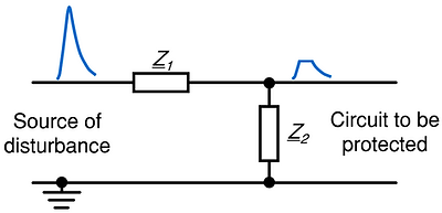
A transient filter stage consists typically of two components (see figure below):

Series impedance Z1. The series impedance limits the transient current through the shunt element and the circuit. Typical series protection components are: resistors, ferrites, or the series resistance and inductance of the conductor itself.
Shunt impedance Z2. The shunt element limits the transient voltage across the circuit. Typical shunt protection components are: clamping devices like TVS diodes and varistors or crowbar devices like thyristors or gas discharge tubes, or simply capacitors.

Shunt protection elements Z2 [Ω] (TVS diodes, varistors, capacitors, etc.) are described in more detail on our webpage about components.

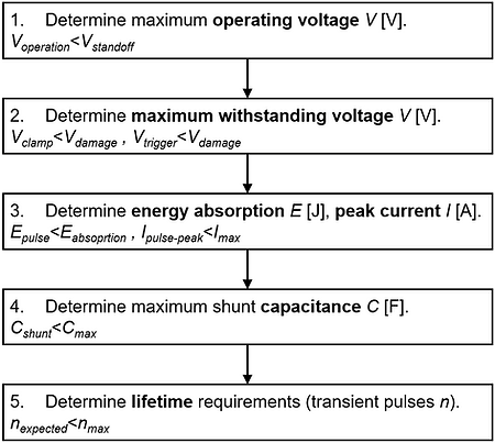
In the following, we focus on the selection of an appropriate shunt protection element Z2 [Ω]. The following points must be considered when choosing a voltage protection shunt element:

Voperation<Vstandoff. The maximum operating voltage must be smaller than the standoff voltage of the shunt element. Up to the standoff voltage (reverse working voltage), the shunt element does not conduct any significant amount.
Vclamp<Vdamage, Vtrigger<Vdamage. With the maximum clamping voltage or the trigger voltage the maximum voltage across the shunt element is meant. This voltage must be lower than the voltage at which the circuit to be protected experiences a defect or malfunction.
Energy absorption: Epulse<Eabsorption. The protective elements must absorb the energy (voltage, current) of the expected transient pulse without any damage.
Signal integrity: Cshunt<Cmax. The protective elements must not interfere with the useful signal (e.g., due to high capacitance or leakage current) and the signal integrity must be guaranteed.
Lifetime: nexpected<nmax. The protective elements must guarantee to withstand the minimum number of expected transient events n during the lifetime, and the protective devices’ degradation must be tolerable.

The points above are summarized in the figure below.

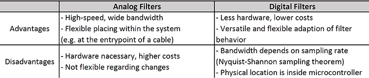
Selecting a protective shunt device for high-voltage transient suppression

Digital Filters

Digital Filters.

Up to this point, all presented filters in this chapter were analog filters. This section is dedicated to digital filters, which have a couple of advantages and disadvantages compared to analog filters (see table below).

Here are some fundamental points about digital filters:

Nyquist-Shannon sampling theorem. In order to convert an analog signal x(t) with the bandwidth B [Hz] (highest frequency in the signal) to a digital signal x[n], a minimum sampling frequency of fs>(2⋅B) [Hz] is required.
Aliasing. Aliasing happens when the Nyquist-Shannon sampling theorem is violated. In order to prevent aliasing, an analog anti-aliasing low-pass filter is placed in front of every ADC. This low-pass filter typically has a cut-off frequency fc [Hz] that is much lower than half of the sampling frequency fs [Hz]: fc<<(fs/2).
FIR-filters. FIR-filters have a finite impulse response (FIR) h[n] and do not have feedback coefficients. Linear moving-average filters are FIR filters.
IIR-filter. IIR-filters have an infinite impulse response (IIR) h[n], use feedback coefficients and provide more design freedom than FIR-filters. Digital filters with Butterworth, Bessel, or Chebyshev behavior require a digital IIR-filter.

The signal flow of an analog signal to an ADC, and finally to a digital filter is shown in the figure below, where fc [Hz] is the cut-off frequency of the analog anti-aliasing low-pass filter, fs=1/Ts [Hz] is the sampling frequency of the ADC.

Even though the usage of digital filters in EMC is limited, they can help improve
robustness, especially when it comes to voltage transient immunity. Here are some
typical examples:

Debounce filter. Analog or digital inputs are read multiple times and checked for unexpected state changes. For example, it could be determined that an input state is only valid when it is stable over a certain period (debounce time).
Analog sensor sanity check. When reading an analog sensor input, e.g., a pressure or a flow rate, the sensor value could be checked if it is within a reasonable range. If not, the sensor value could either be reread, or the system could throw a warning.
Input states sanity check. In the case of multiple sensors (e.g., position sensors along a linear drive with a slider), a sanity check could be performed (e.g., it is only possible that one single position sensor along the linear drive detects the slider). In the event of an implausible result, a new status query could be triggered, or the system could enter a safe state.
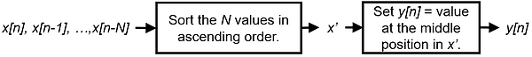
Median filter. Median filters are non-linear filters that provide a reliable way to get rid of short spikes and dips in an input signal. The filter takes an array of N values, sorts it in ascending order, and returns the value in the middle of the sorted array.

Spike-remover. A spike remover detects a spike in an array of data and replaces the spike data with valid data points. The figure below shows the principle of a single data point spike-spike remover.

References:

[13.1] Dimitry Gorinevsky. Lecture Notes for EE392m, Control Engineering in Industry:
Linear Systems. Stanford University, Information Systems Laboratory
Department of Electrical Engineering, 2005.

[13.2] Reto B. Keller, Design for electromagnetic compatibility - In a nutshell, Springer, 1st Edition, 2023, p. 256

Academy of EMC

Education for professional engineers.

13 Filtering