
Antenna Fundamentals.
An antenna is an interface between radio waves propagating through space and electric currents moving along metal conductors. It can act as a receiver (converting electromagnetic waves from space into voltages and currents in a conductor) or as a transmitter (converting voltages and currents into electromagnetic waves).
Isotropic Radiator and Power Density S.
First, we need to introduce two terms: isotropic radiator and power density S [W/m^2]. An isotropic radiator (isotropic antenna) radiates equally in all directions (from one single point) and therefore has no directivity. Such an antenna does only exist in theory. S represents the power density of the field around an antenna at a given distance d. The power density S of an isotropic radiator is simply the radiated power Prad by the antenna [W] divided by the surface area of the sphere [m^2] with the distance d [m] from the center of the radiator [7.1].

The power density Sw [W/m^2] of a plane wave is defined as the product of the E-field [V/m] and H-Field [A/m]. ZW is the wave impedance 120π = 377 [Ω].
Antenna Gain G.
In EMC testing, we use directional antennas (e.g. biconical dipole antennas, horn antennas) which have an antenna gain G. The antenna gain G [1] ([dB]=log10(G[1])) is defined as the ratio of the power radiated in the desired direction of an antenna compared to the power radiated from a reference antenna (e.g. isotropic radiator or dipole) with the SAME power input (this means the antenna efficiency factor η=Prad/Pt, which considers the antenna losses, is already taken into account in gain G) [7.2]:

The antenna gain Gi of an ideal halve-wave (λ/2) dipole is 1.64 [1] (2.15 [dBi]), whereas the antenna gain Gd of an ideal halve-wave (λ/2) dipole is 1 (0 [dBd]) [7.2]:

The antenna gain compared to an isotropic radiator Gi and the antenna gain compared to a dipole antenna Gd are in the following relation to each other [7.2]:

Now, we are ready to calculate the often used terms: effective isotropic radiated power (EIRP, referred to as an isotropic radiator) and effective radiated power (ERP, referred to a λ/2-dipole) [7.3]:

Pt = transmitter antenna input power [W], Gi = antenna gain referred to a isotropic radiator [1], Gd = antenna gain referred to an ideal λ/2-dipole [1]. The power density S [W/m^2] at a distance d [m] from the transmitter antenna can now be written as:
Effective Aperture Ae.
Another useful parameter to know is the effective area of an antenna, also called effective aperture Ae [m^2]. The effective aperture represents the ratio of power Pr [W] (output power of the receiver antenna) to the power density SW [W/m^2] (power density of the plane wave which reaches the antenna) [7.2]:

The maximum effective aperture Aem [m^2] for any antenna can be calculated by multiplying the squared signal wavelength λ [m] with the antenna gain Gi and dividing it by 4π. The maximum effective aperture Aem [m^2] refers to the circumstance where the load impedance is the conjugate of the antenna impedance (matched impedances, which means that the maximum power transfer to the load takes place) and the incident wave and the polarization of the antenna are matched.

Antenna Factor AF.
The antenna factor AF [1/m] or [dB/m] is the term that is often needed during EMC emissions testing. AF is used to calculate the received field strength E [V/m] based on the measured voltage Vr [V] at the receiver's antenna terminals. We focus on the antenna factor of E-field antennas. Therefore the antenna factor is the ratio of the strength of the electric field E [V/m] at the antenna to the voltage Vr [V] at the terminals of the receiver antenna [7.4]:

Now, we have everything ready to express AF [1/m] or [dB/m] as a function of only the plane wave frequency f [Hz] and the receiver antenna gain Gir [1] (in case of matched impedances and aligned antenna to the polarization of the incident wave):
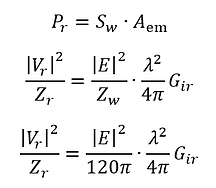
Vr = voltage at receiver antenna terminals [V], Zr = impedance of receiver [Ω] (typically 50 [Ω]), E = field strength of plane wave [V/m], λ = wavelength of plane wave signal, Gir = receiver antenna gain referred to an isotropic antenna [1], ZW = plane wave impedance [Ω] (377 [Ω] for far field), Aem = maximum effective aperture [m^2]
If we rearrange the formula from above and replace λ=c/f (c=3E8[m/sec]), we get AF as a function of f, Zr and Gir:

AF is often used in [dB/m]:
Replace the wavelength λ=c/f, where c=3E8 [m/sec]. Now, we can express AF [dB/m] as a function of signal frequency f in [MHz] (!), receiver antenna gain Gir, and impedance at receiver measurement instrument Zr [Ω]:
7 Antennas
This chapter is a brief introduction to the topic of antennas and electromagnetic radiation. We skip the math intense part around the Maxwell Equations. The formulas and statements in this chapter are applicable to the far-field / free-space (not the near field), matched impedances (of antennas and receiver/transmitter equipment) and matched polarization (of the electromagnetic waves and the antenna polarization).
Antenna Formulas: Emission Testing.
We focus here on EMC emission testing like CISPR 11 or CISPR 32. In other words: the physical quantity of interest is the E-field [dBμV/m] and the measured physical quantity is the voltage Vmeasure [dBμV] at the EMI receiver or spectrum analyzer (for [dBm] to [dBμV] conversion: look here).
When we set the receiver impedance Zr to 50 [Ω] and wavelength λ=c/f (c=3E8 [m/sec]), we get this for the receiver antenna factor AF:

The field strength E [V/m] at the antenna can be calculated based on AF [1/m] (which is frequency-dependent!) and Vr [V] (output voltage from the receiver antenna):
Let's consider the cable loss [dB] from the antenna to the measurement instrument (EMI receiver, spectrum analyzer) and call the measured voltage at the receiver Vmeasure [dBμV]. Thus, we can calculate the strength of the E-field [dBμV/m], based on the receiver's antenna factor AF [dB/m], the measured voltage at the receiver Vmeasure [dBμV], and the cable loss [dB]:
Antenna Formulas: Immunity Testing.
We focus here on EMC immunity testing like IEC 61000-4-3. In other words: the physical quantity of interest is the E-field [V/m] at a certain distance d [m] for a given transmitter antenna input power [W].
From the antenna fundamentals above, we know how to calculate the power density S [W/m^2] at a distance d [m] for a transmitter antenna with an antenna gain Git [1] and the power Pt [W] at the transmitter antenna terminals:
Furthermore, we know the power density S [W/m^2] of a plane wave in free space (far-field characteristic impedance of Zw=120π [Ω]) is given by [7.1]:

If we combine these two formulas above, we can determine the field strength E [V/m] at a given distance d [m] from the antenna for a given transmitter antenna input power Pt [W]:

The required power input power of a transmitting antenna Pt [W] for achieving a desired field strengt E [V/m] at a given distance d [m] is:

Unintended Antennas.
Current loops, PCB structures, cables, or slots may act as unintended antennas. As
a result, they receive or emit electromagnetic radiation unintentionally.
E-Field From Differential-Mode Currents In Small Loops.
Let us assume a setup like the one shown in the figure below, where the following is given [7.6]:
-
Electrically small current loop (circumference < λ=4), so that the current distribution (magnitude, phase) is constant along the current loop.
-
The measurement point of the E-field is in the far-field.

Given the points above, the maximum electric field EDMmax [V/m] caused by a differential-mode current IDM [A] can be approximated as [7.6]:

where, EDMmax = maximum RMS field-strength radiated by electrically small current loop with area A and differential current IDM in [V/m], IDM = RMS value of the differential-mode current in [A], f = frequency of the sinusoidal current signal in [Hz], A = area of the current loop in [m2], d = distance to the center of the current loop in [m].
E-Field From Common-Mode Currents In Short Cables.
Let us assume a setup like the one shown in the figure below, where the following is given [7.7]:
-
Electrically short cable length l [m] (e.g. l < λ=4), so that the current distribution
(magnitude, phase) is constant along the conductor.
-
The measurement point of the E-field is in the far-field.

Given the points above, the maximum electric field ECMmax [V/m] caused by the common-mode current ICM [A] can be approximated as [7.7]:

Maximum E-Field From Common-Mode Signals.
When the cable length l [m] approaches λ/4 the cable starts to become a good radiator. Radiated emissions are worst at cable length l = nλ/4, where n is [1, 2, 3, ...] because the cable is at resonance at these lengths.
-
Maximum E-Field For A Given Common-Mode Current ICM [A]. Assuming a common-mode current ICM [A] flows along a resonant structure (e.g. a cable). When in resonance (and only then!), the maximum electric field strength Emax [V/m] can be approximated as [7.8]:

where Emax [V/m] is the maximum RMS E-field at distance d [m] for matched impedances, matched polarization, line-of-sight path, and a resonant structure driven by ICM [A], ICM [A] is the RMS common-mode current that flows along the resonant structure, Rrad [Ω] is the radiation resistance (λ/2-dipole: 73Ω, λ/4-monopole: 36.5Ω), η0 [Ω] is the intrinsic impedance of free-space (120π Ω) and Gi [1] is the antenna gain (λ/2-dipole, 1.64; λ/4-monopole, 3.28).
If we set Rrad = 73Ω and Gi = 1.64 for a λ/2-dipole and Rrad = 36.5Ω and Gi = 3.28 for a λ/4-monopole, we get [7.8]:

-
Maximum E-Field From A Given Common-Mode Voltage VCM [V]. Assuming a common-mode voltage VCM [V] drives a resonant structure (e.g. a cable). When in resonance (and only then!), the maximum electric field strength Emax [V/m] can be approximated as:

where Emax [V/m] is the maximum RMS E-field at distance d [m] for matched impedances, matched polarization, line-of-sight path, and a resonant structure driven by VCM [V], VCM [V] is the RMS common-mode voltage that drives the resonant structure, Rrad [Ω] is the radiation resistance (λ/2-dipole: 73Ω, λ/4-monopole: 36.5Ω), η0 [Ω] is the intrinsic impedance of free-space (120π Ω) and Gi [1] is the antenna gain (λ/2-dipole, 1.64; λ/4-monopole, 3.28).
If we set Rrad = 73Ω and Gi = 1.64 for a λ/2-dipole and Rrad = 36.5Ω and Gi = 3.28 for a λ/4-monopole, we get:

References:
[7.7] Clayton R. Paul. Introduction to electromagnetic compatibility. John Wiley & Sons Inc., 2nd Edition, 2008, p. 515